
Executive Summary
The Contrastive Credibility Propagation (CCP) algorithm is a novel approach to semi-supervised learning (SSL) developed by AI researchers at Palo Alto Networks to improve model task performance with imbalanced and noisy labeled and unlabeled data. This post is based on our paper, published and presented at The 38th Annual AAAI Conference on Artificial Intelligence (AAAI ‘24). The paper shows that CCP expands robustness to five different data quality issues often found in real-world datasets compared to several state-of-the-art SSL algorithms.
This research better supports practitioners building classifiers with these kinds of datasets. This can help unlock the usefulness of unlabeled data, which is often more abundant and task-relevant but may be too messy for known methods only previously demonstrated to work on clean datasets.
In addition to summarizing the paper at a high level, we illustrate an example of applying CCP to the critical cybersecurity task of machine learning (ML) powered data loss prevention (DLP). DLP is well suited to demonstrate CCP’s unique benefits as real-world DLP traffic is noisy and unviewable due to privacy concerns. Specifically, we focus on building an ML classifier to differentiate sensitive versus non-sensitive text documents. The model also identifies what kind of sensitive data is contained in a sensitive document (e.g., medical information, financial accounting documents, lawsuit proceedings, or source code). We explain how to apply CCP to a DLP deep neural network (DNN) classifier. This is followed by demonstrating the overarching goal of reducing the loss of classification accuracy when moving from a curated test set to real-world data.
Palo Alto Networks customers are better protected from the threats discussed in the above research through our Cloud-Delivered Enterprise DLP product.
| Related Unit 42 Topics | Machine Learning |
Introduction to CCP
Research Question
SSL leverages both labeled and unlabeled data to train a single model. Often, people use SSL to build a classifier (i.e., a model that decides for each sample what class it belongs to from a predefined set of classes).
In this context, a labeled sample means we know in advance what class that sample belongs to, and unlabeled means we do not. However, we can often still extract useful information from the unlabeled data to build a better classifier as indicated in Figure 1. That is what SSL algorithms are designed to do.
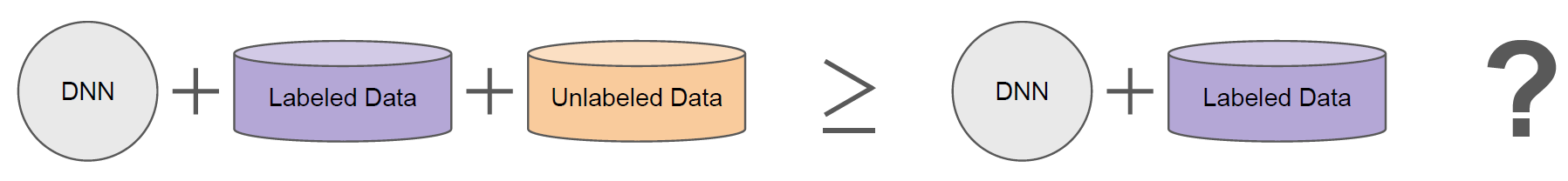
However, it’s not uncommon for a model trained with SSL to perform worse than one trained only on labeled data (i.e., fully supervised).
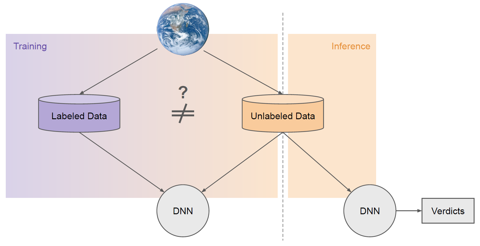
As illustrated in Figure 2, a common reason for this is that the labeled and unlabeled datasets often have distinct properties. They are often sampled from different sources (i.e., distributions).
For example, labeled datasets are typically collected manually offline by practitioners and annotators. Unlabeled data, on the other hand, typically comes from the same source you wish to deploy your model on in the real world.
One of the core motivations of SSL is aligning models to real-world distributions that are too plentiful or messy to label. Curated labeled datasets often take on distinct characteristics from unlabeled data.
By the nature of being unlabeled, the relative frequency of classes in real-world data is typically unknown or even unknowable. Sometimes, unlabeled data is unviewable due to privacy concerns or in the deployment of fully autonomous systems.
More examples of data quality issues are as follows:
- Concept drift within classes (e.g., change in the prototypical example of a class).
- Unlabeled data containing data that belongs to no class
- Errors in the given labels
SSL algorithms are seldom equipped to handle these quality issues, especially combinations thereof. In literature, this often goes unnoticed as, in many works, the sole experimental variable is the number of labels given on otherwise clean and balanced academic datasets.
Our research question is this: can we build an SSL algorithm whose primary objective is to match or outperform a fully supervised baseline for any dataset?
Core Algorithm Components
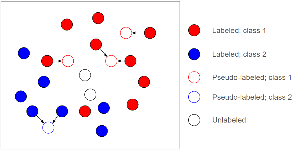
SSL comes in many flavors. A common, powerful approach is to generate and leverage what are known as pseudo-labels for unlabeled data during training. Illustrated in Figure 3, pseudo-labels are (often soft) labels produced dynamically for unlabeled data during training that are then used as new supervision sources for further training.
In the best-case scenario, if all pseudo-labels are correct, it can be as powerful as if all the unlabeled data were labeled. This is, of course, unrealistic.
It's common for the true class of unlabeled data to be indiscernible from the given label information. This means pseudo-labels will inevitably have errors, which is why pseudo-label approaches are also inherently dangerous. SSL algorithms, especially those implemented with deep neural networks, tend to be very sensitive to these errors in pseudo-supervision.
To approach our research question, we start with a simple assumption: pseudo-label errors are the root cause of SSL algorithms failing to match or outperform a fully supervised baseline. Intuitively, without those errors, an algorithm should have no issue at least matching the fully supervised baseline.
CCP is designed around this principle. Specifically, we aim to build an SSL algorithm that is foremost robust to the pseudo-label errors that it inevitably produces.
Iterative Pseudo-label Refinement
Learning with noisy labels is a rich field of research. For CCP, we draw inspiration from prior works in this space.
There is an important distinction between class-conditional label noise and instance-dependent label noise. Instance-dependent label noise refers to the type of noise where the probability of label errors depends on the specific characteristics (features) of the instance.
Class-conditional label noise, on the other hand, refers to label errors that are dependent on the true label. Pseudo-label noise is highly instance-dependent as each pseudo-label is generated dynamically on a sample-by-sample basis. This narrows down our search further.
A powerful method previously demonstrated on fully supervised problems is called a self-evolution average label also known as SEAL. The main idea is to train a model with noisy labels and to produce new predictions for every data sample multiple times throughout the training process. You then average those predictions together to produce the next set of labels you’ll use in the next iteration. This works because, in the presence of an incorrect label, your model will often oscillate its prediction between the correct and incorrect class before it typically memorizes the incorrect class late in training.
Averaging those predictions across time slowly pushes the label in the right direction. A similar pattern in pseudo-label oscillations was observed in our study. An example of pseudo-label oscillation is shown in Figure 4.
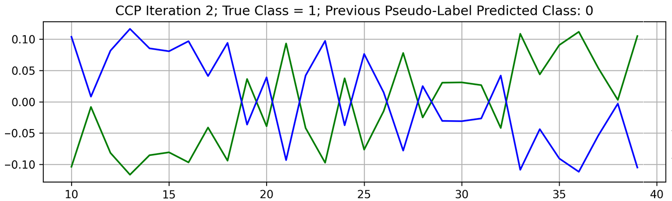
Early in training, when the model has not overfitted to the wrong label, the score for the true class is high. This is reversed when the model has time to fit itself to the wrong label.
CCP features an outer loop designed to exploit this phenomenon, illustrated in Figure 5. For every batch of data during training, we predict new pseudo-labels for unlabeled data, then average them together to mark the end of an iteration.
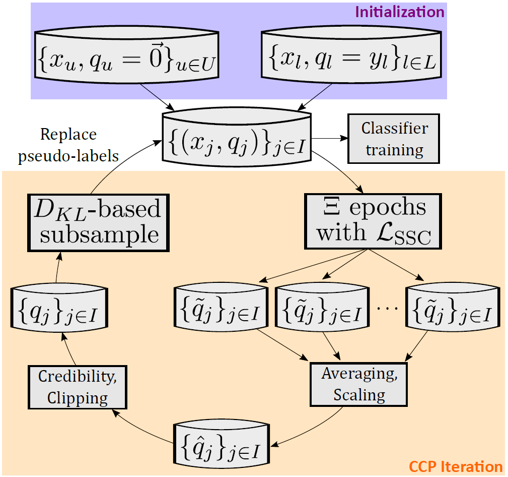
These “CCP iterations,” designed to refine pseudo-labels iteratively, take place strictly before a classifier is ever built. The pseudo-labels are generated transductively, meaning we infer each sample based only on other samples in the batch.
Classifiers are inductive and try to learn generalizable patterns across all data. Importantly, these noisy, batch-level, transductive pseudo-labels are never directly used to supervise our inductive classifier. We clean the pseudo-labels through iterative refinement first.
Credibility Representations
As mentioned previously, it's common for the true class of unlabeled data to be indiscernible from the given label data. This may be due to ambiguity or gaps in the label information.
We’d ideally like to discard pseudo-label information for those samples or otherwise nullify their impact on learning. We adopt a label representation called “credibility vectors” that allows us to do the former.
Traditionally, label vectors are computed via a softmax function. This function transforms a vector of real values (class scores or similarities) into a vector of values all in the range [0, 1] that sums to 1 such that they can be interpreted as probabilities.
The function preserves the ranking of values (i.e., small input values will correspond to small output values and vice versa). Credibility transforms an input vector of class scores/similarities with range [0, 1] into an output vector with range [-1, 1].
In a credibility vector, -1 corresponds to high confidence in class dissimilarity, 0 corresponds to no confidence either way and 1 corresponds to high confidence in class similarity. The core idea of credibility is to condition class similarity measurements on the next highest class similarity (i.e., a large class similarity measure only remains high if no other class similarity measures are also large).
Consider the example in Figure 6.
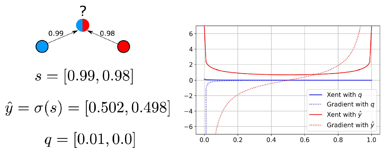
On the left of Figure 6, we see an unlabeled sample with large class similarity scores of 0.98 and 0.99 to the red and blue classes, respectively. The true label is nearly ambiguous. The softmax label is computed as [0.502,0.498]. The credibility vector is computed as 0.99-0.98=0.01 in the first entry and 0.98-0.99=-0.01 in the second entry (which is clipped to 0).
In SSL, these pseudo-labels are often used to supervise an underlying model with a classification loss. We can see the effect of using each on the standard classification loss function called cross-entropy (Xent) on the right of Figure 6.
In that plot, consider the X-axis the softmax output of a binary classifier for the blue class. Computing cross-entropy with the softmax label induces a strong gradient at either pole despite the true class being nearly ambiguous.
Using the credibility label will ensure the gradient for this sample is near 0 everywhere except for x=0. Where all classes are equally similar, the credibility label would be the zero vector and the gradient would be zero everywhere. This representational capacity is important because we often view incorrect pseudo-labels improving through CCP iterations sometimes just by shrinking in magnitude (e.g., when the true class is indiscernible).
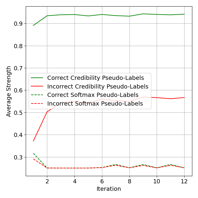
In an ablation analysis in Figure 7, we see a key benefit of credibility representations is differentiating correct versus incorrect pseudo-labels. On average, the strength (maximum value) difference between correct and incorrect pseudo-labels is much greater when using credibility. This is likely due to its more strict criteria for assigning large scores. It is thus a better measure of confidence.
The entire CCP framework, from pseudo-label refinement to classifier building, makes native use of credibility and the better differentiation it provides. Through weighted averages, a sample’s impact on label propagation and all loss functions scales linearly with the magnitude of the single non-zero entry of a credibility label. Zero vectors also provide a natural initialization for pseudo-labels in the first CCP iteration.
Subsampling
Figure 7 suggests that the strength of credibility labels is effective at identifying pseudo-labels that are incorrect. Naturally, one may ask if we can use this signal to refine the pseudo-labels during CCP iterations further. We define a subsampling procedure that does just this.
This procedure is optional, but it does help speed up convergence and even converge at better solutions with generalizable settings. At the end of an iteration, we compute a percentage of the weakest pseudo-labels to reset back to their initialization (the zero vector). This allows the network to train on a cleaner pseudo-label set for the next iteration. Reset pseudo-labels will be assigned a new pseudo-label in the next iteration.
What percent of the weakest pseudo-labels should we reset? Resetting too many pseudo-labels can lead to instability in training (i.e., the accuracy of pseudo-labels dropping rapidly or failing to converge across iterations).
We hypothesize that the cause of this instability is similar to the cause of instability observed with self-training techniques. Self-training is the concept of iteratively assigning unlabeled data pseudo-labels and moving them (usually the strongest ones) into the train set. Many state-of-the-art SSL algorithms can be categorized as a form of self-training.
Here, we are resetting existing pseudo-labels that would otherwise be kept. So, in a sense, it’s the inverse of self-training.
A unique strength of CCP is that it is highly stable without subsampling (a theoretical explanation for this is provided in the paper). This awards us a path to balance stability with the desire to reset incorrect pseudo-labels. We consider a wide range of candidate subsampling percentages of the weakest pseudo-labels to reset.
We first compute a probability distribution over classes that summarizes the state of all pseudo-labels in totality (sum them together then divide by the total mass). This serves as our anchor distribution – it's what we want to limit the divergence from.
For each candidate subsampling percentage, we compute a summarizing probability distribution over the pseudo-labels again after resetting the weakest corresponding percent of pseudo-labels. We then have a new summarizing probability distribution for each candidate subsampling percentage.
We compute the Kullback-Leibler divergence (the difference in information between probability distributions) of each candidate distribution from the anchor distribution. These divergence measures represent how much the summarizing probability distribution changes when increasing the candidate subsampling percentage.
To finish subsampling, we simply choose the highest candidate subsampling percentage that obeys a strict limit on the divergence and then apply that to our pseudo-labels. We slowly decrease the strict cap on divergence through CCP iterations to support convergence.
Importantly, this method is free of imposing assumptions and normalized to the dataset size. Accordingly, a single subsampling schedule generates well across all of our experiments.
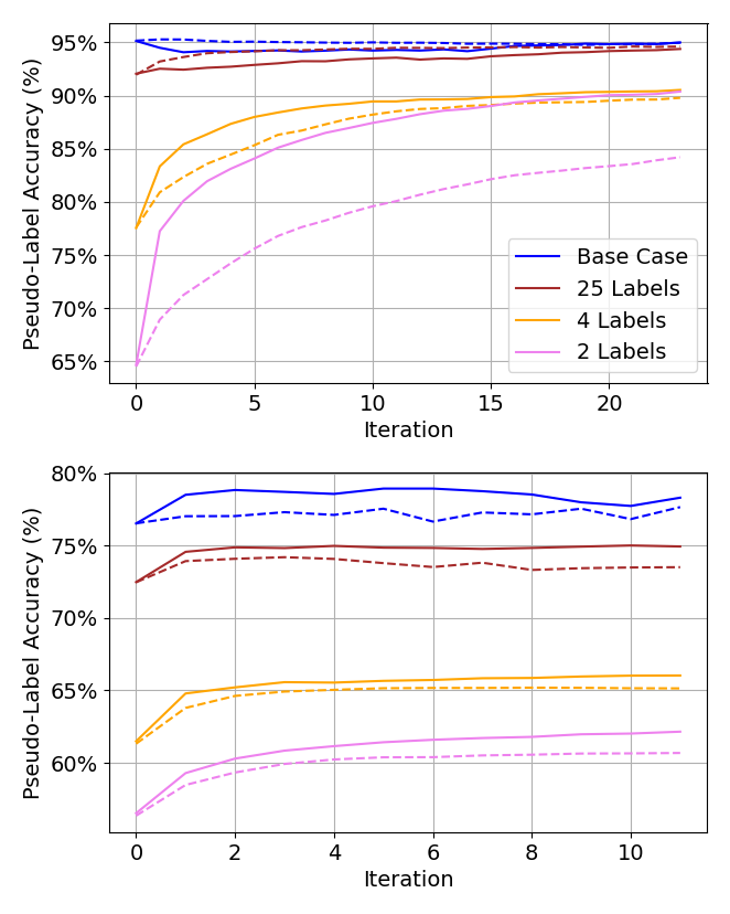
Examples of an ablation study on subsampling are shown in Figure 8. Specifically, we see the state of pseudo-labels converge faster and the overall accuracy of pseudo-labels increase upon convergence.
Experimental Results
Our paper has a comprehensive overview of all our experimental results. We enumerate five different kinds of data quality issues (data variables) and then measure the sensitivity of five state-of-the-art SSL algorithms to these data variables.
Sensitivity refers to how big of an impact a data variable has on the results of an SSL algorithm. The five data variables in question are:
- Few-shot: Changing the scarcity of labeled data.
- Open-set: Changing the percentage of unlabeled data that belongs to no class.
- Noisy-label: Changing the percentage of given labels that are incorrect.
- Class imbalance/misalignment: Changing the class frequency distributions in the labeled and unlabeled sets separately (while the other remains balanced).
Each algorithm tested was optimized for a single, specific data variable. However, as we argue here, a practitioner rarely knows in advance what data variables they need to overcome. There is thus a gap in the practical usefulness of narrowly optimized methods.
We explore each data variable at three levels of severity. We construct our data variable scenarios by applying corruptions to two standard benchmark computer vision datasets (CIFAR-10 and CIFAR-100). In addition to our SSL algorithms, we train a supervised baseline in every scenario.
In brief, CCP is not the optimal solution for every scenario, but it demonstrates remarkable consistency. For example, it is the only algorithm outperforming the supervised baseline in every scenario.
We discovered one or more scenarios that result in catastrophic performance degradation for every other algorithm. This is shown in Table 1, which distills the minimum accuracy of each algorithm on our two datasets across all scenarios.
| Algorithm | CIFAR-10 | CIFAR-100 |
| CCP (Ours) | 90.23% | 61.38% |
| CoMatch | 50.05% | 47.94% |
| ACR | 39.75% | 22.07% |
| OpenMatch | 43.08% | 27.88% |
| FixMatch w/o DA | 44.62% | 41.84% |
| FixMatch w/ DA | 46.97% | 40.95% |
Table 1. Minimum accuracies for each algorithm across all scenarios for both datasets.
CCP Applied to DLP
DLP is a critical cybersecurity task aimed at monitoring sensitive data within an organization and preventing its exfiltration. ML-powered DLP services feature models that must autonomously classify if a given document is sensitive or not sensitive. Often, models must also determine what kind of sensitive data lies within the document (e.g., financial, health, legal or source code).
For this demo, we apply CCP to a similar deep learning DLP classifier. To simplify, we assume the input document contains only text. However, CCP applies to any model tasked with ingesting documents of any modality. The demo document classifier recognizes multiple sensitive document classes and one non-sensitive class.
A practitioner faced with building such a classifier must overcome some fundamental challenges. By definition, the data you’d like to classify in deployment is unviewable due to privacy concerns.
Labeled datasets to train, test and validate a classifier must be gathered with publicly available versions of sensitive documents or custom synthetic samples. Both of those efforts are useful, but, in any non-trivial deployment scenario, there will inevitably be a large information gap between labeled data and production data.
The class frequency and content frequency distributions may vary widely. Also, new types of content for a given class may be present in production data but not in your labeled dataset. Naturally, the desire to train on real production data arises.
The rough sketch of applying CCP to a DLP classifier is as follows:
- We define a means to extract privatized versions of unlabeled sensitive production data
- We attach the lightweight architectural components necessary to compute CCP’s algorithms and losses to the existing classifier
- We repeat CCP iterations to iteratively refine a set of pseudo-labels for all the unlabeled data
- We use a combination of given labels and the final state of pseudo-labels to train a final inductive classifier
Working with Sensitive Data While Preserving Privacy
Many solutions have been proposed to train with private data. Popular solutions include federated learning, homomorphic encryption and differential privacy (DP).
A comparative discussion of these techniques is out-of-scope for this blog. We instead detail how one can use a combination of DP and CCP to train on production data in a privacy-preserving yet effective manner.
To understand DP, consider the following. Imagine you’re in a classroom and you have a secret – your favorite food is broccoli, but you don't want anyone to know. Now, suppose your teacher is taking a survey of everyone's favorite food in class. You don't want to lie, but you also don't want anyone to know your secret. This is where DP comes in.
Instead of telling your true favorite food, you decide to flip a coin. If it's heads, you tell the truth. If it's tails, you pick a food at random.
Now, even if your teacher says “someone in class likes broccoli,” no one will know for sure it's you, because it could have been a random choice. DP works similarly. It adds a bit of random "noise" to the data. The noise is enough to keep individual information private, but not so much that the overall trends in the data can't be seen.
Your teacher can still get a general idea of the class's favorite foods, even if they don’t know that you secretly love broccoli. The key aspect here is that by introducing the coin flip (or randomness), you're adding an element of plausible deniability.
Even if someone guessed that you chose broccoli, the coin flip introduces doubt, protecting your privacy. In the context of DLP document classification, we use DP to preserve the privacy of production documents while mostly preserving the general statistics of a large collection of documents.
We need a real-valued representation of the document to apply DP noise to and achieve its theoretical privacy guarantees. A special feature extraction model is typically used for this purpose. Its job is to non-reversibly convert a text document into a large collection of floating point numbers.
This representation is unreadable by a human but preserves the high-level semantics of the document (an additional layer of privacy). Industry-standard levels of DP noise are added to this floating point representation to ensure the representation can be safely extracted from production data.
Despite having privatized representations of sensitive documents, you must still overcome the fact that the representations are unlabeled. This is where CCP comes into play.
Neural Architecture Details
Our deep learning model takes in privatized representations of documents as input. Its task is to output the correct classification verdict for each input sample.
CCP also requires us to define a separate embedding space within which we will learn a similarity function that compares inputs. The similarity function will be trained to assign inputs of the same class with higher similarity than inputs of different classes.
This similarity function is trained with a contrastive loss allowing us to produce pseudo-labels transductively. The core architecture components of CCP are illustrated in Figure 9.
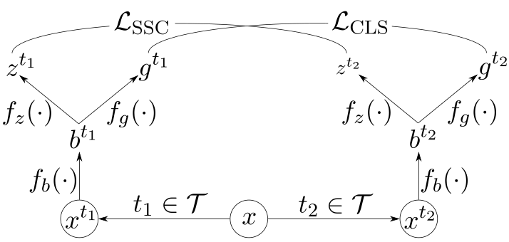
The notation in Figure 9 is as follows:
- \(x\) – An input sample
- \(\mathcal{T}\) – The set of transformations
- \(t\) – A randomly sampled transformation
- \(f_b\) – The encoder network
- \(f_z\) – The contrastive projection head
- \(f_g\) – The classification projection head
- \(\mathcal{L}_{\text{SSC}}\) – Softly supervised contrastive loss
- \(\mathcal{L}_{\text{CLS}}\) – Standard cross-entropy classification loss
Firstly, in line with other work on contrastive learning, we define a set of transformations, \(\mathcal{T}\), over our data. The job of transformations is to corrupt the low-level details of an input while preserving its high-level class semantics.
For images, this could be random crops or color jitter. For text, this could be noise added to the embedding vectors or randomly hiding words.
Randomly drawing two transformations leads to two views of each input sample with the same class label. These transformations help the learned similarity metric and the classifier robustly overcome low-level noise.
An encoder network, \(f_b\), processes the transformed batch of data. The encoder’s job is to transform the input into a new encoded vector space.
The exact structure of \(f_b\) (a CNN, transformer, RNN, etc) depends only on what makes sense for your datatype. A transformer would be a common choice for DLP and natural language documents.
Two projection heads (\(f_z\) and \(f_g\)) bring the encoder outputs into two new vector spaces upon which we compute our loss functions. Each projection head is a multilayer perceptron (i.e., a short sequence of fully connected layers).
Concerning an existing deep learning DLP classifier, \(f_g\) would be the last layer of your classifier (upon which you compute softmax and your classification loss) while \(f_b\) would be everything prior. The \(f_z\) projection head, used to learn a similarity metric, would be the only new neural network component to add.
Learning and Applying a Similarity Metric
The algorithms and losses unique to CCP are computed within the vector space defined by \(f_z\). We define a novel contrastive loss to learn the similarity metric that is softly supervised.
Two popular contrastive loss functions are SimCLR and SupCon, which can be interpreted as unsupervised and supervised versions of the same loss. Both loss functions assume that positive and negative pairs are sampled discretely (pairs that should be similar and dissimilar, respectively). This is not the case when we have soft pseudo-labels. We only have variable confidence of positive pair relationship defined by the magnitude of the pseudo-label vector.
We describe a generalization of SimCLR and SupCon designed to work with this uncertainty, denoted \(\mathcal{L}_{\text{SSC}}\). Our study shows that SimCLR and SupCon losses are special cases of \(\mathcal{L}_{\text{SSC}}\).
Following the formalization of the algorithm visualized in Figure 5, we repeat the cycle of propagating pseudo-labels with this learned similarity metric followed by averaging pseudo-labels across epochs. We apply subsampling as defined above as necessary.
Once the process has converged, we use the final state of pseudo-labels to train a new inductive classifier consisting of \(f_b\) and \(f_g\). In practice, retaining \(f_z\) to compute \(\mathcal{L}_{\text{SSC}}\) during classifier training as an additional loss provides a classification performance boost. However, during inference, \(f_z\) is discarded.
Impact
We outline above the steps to train a DLP classifier on a combination of a curated labeled dataset and unlabeled, privatized production data with CCP. By doing so, you’ve made an important step toward aligning your machine learning model with your target production data distribution.
Despite achieving similarly high test set classification performance in internal experiments, DLP classifiers adjusted with CCP saw a 250% increase in successful detections of sensitive documents in a real-world test. This underscores the critical importance of ensuring the alignment of your ML models to the actual deployment data distributions. Traditional performance metrics on a test split of your curated dataset can sometimes be very misleading!
CCP provides a useful tool for practitioners to confidently align models when the deployment data distribution is unlabeled or even unviewable. DLP is just one experimental setting. CCP is general enough to provide value for any classifiers built on any partially labeled dataset.
Conclusion
We have reviewed the CCP algorithm, its core components and some benchmark analyses presented in depth at AAAI ‘24. We have discussed its specific, unique benefits compared to other semi-supervised learning algorithms.
We’ve walked through an example of applying CCP to DLP, a critical component of any enterprise cybersecurity solution. We’ve discussed why DLP is well suited to demonstrate CCP’s unique strengths.
Palo Alto Networks continues to improve state-of-the-art DLP. Enterprise DLP customers are better protected against sensitive data loss through CCP.
Additional Resources
- Contrastive Credibility Propagation for Reliable Semi-Supervised Learning – Brody Kutt, Pralay Ramteke, Xavier Mignotar et. al. on arXiv
- A Simple Framework for Contrastive Learning of Visual Representations – SimCLR on GitHub
- Supervised Contrastive Learning – Prannay Khosla, Piotr Teterwak, Chen Wang et al. on arXiv
- Self-Training: A Survey – Massih-Reza Amini, Vasilii Feofanov, Loic Pauletto et al. on arXiv
- Differential Privacy – Wikipedia
- Homomorphic Encryption – Wikipedia
- Federated Learning – Wikipedia
- Kullback-Leibler Divergence – Wikipedia
- Cross-Entropy – Wikipedia
- Softmax Function – Wikipedia
- Statistical Classification – Wikipedia
- Semi-Supervised Learning – Wikipedia
- Data Loss Prevention – Palo Alto Networks
- The 38th Annual AAAI Conference on Artificial Intelligence
- CIFAR-10 and CIFAR-100 – Alex Krizhevsky, Learning Multiple Layers of Features from Tiny Images.
Updated June 28, 2024, at 9:55 a.m. PT to correct the text.
Table of Contents
Related Threat Research Resources